WELLOG INDUCTION LOG

THE INDUCTION LOG:

Conventional electric logging requires a conductive path for current to flow. When oil based muds are used for drilling a well, there may be little or no conductive fluid in the borehole. The induction log overcomes the need for conductive fluid. It will operate in oil based mud, water, or air drilled holes.

THE INDUCTION METHOD:

The induction method utilizes an electromagnetic transmitter coil to generate an alternating magnetic field. The alternating magnetic field induces current flow in the surrounding earth and the induced currents generate a secondary alternating magnetic field. A second coil called a receiver coil is located in close proximity to the transmitter and on the same axis. The secondary magnetic field (earth loop) is changed in amplitude and phase by the surrounding electrical properties of the earth. View induction tool schematic.

PROPAGATION AND SKIN DEPTH:

Inductive methods are best described as transformer coils linked by their mutual inductances. Electromagnetic energy coupling the loops undergoes attenuation and phase shift as it propagates. Skin Depth is a measure of the distance to which an electromagnetic wave will penetrate. Skin depth is a function of frequency and resistivity. The more conductive the medium the larger the currents and the shorter the distance over which the electromagnetic wave can penetrate.

Skin Depth = d = (2/mwC)¹^/2

Where:

Permeability = m = Newtons per ampere squared (SI) dimensionless (cgs)

Angular frequency = w = 2 * p * F

Conductivity = C = Siemens per meter (Note: S replaces the older mho)

Example:

Permeability = 1 (air), Frequency = 20,000 Hz, and resistivity = 100 ohm-meters ( C = 1/100 = .01 mho-meters)

Skin depth = 50 meters

INDUCTION NUMBER:

We can represent the electrical properties of an elementary loop by discrete circuit elements i.e. resistance R in ohms and inductance L in Henries. In this case the earth loop is considered to be a coil that creates the secondary magnetic field.

For a single turn loop:

Induction Number = θ = wL/R

NORMALIZED SIGNAL:

The normalized signal is the product of two terms. The first term is called the radial geometric factor. It incorporates only the distances between the coils and the loop. The second term is called the induction factor. It depends only upon the properties of the elemental loop as given by the induction number. The induction factor is complex-valued. The received voltage consists of components which are in phase and out of phase with the transmitting coil. At large values of induction number, the in-phase component dominates. At small induction numbers, the out of phase component becomes more dominant. Induction tools sense the out of phase (Quadrature) signal using a phase sensitive detector.

Radial geometric factor example:

The medium induction tool derives ____ percent of its signal from within 80 inch diameter?

View high resolution radial geometric factors chart.

FOCUSED INDUCTION TOOL:

At small induction numbers, the transmitter signal can be orders of magnitude greater than the desired signal. It is common practice to null out the primary field by coil arrange. It is also common practice to use supplementary coils to cancel the contribution of the field above and below the main coils and reduce the near-borehole field allowing more penetration into the formation.

View a focused induction tool schematic.

Full solution for homogeneous medium:

In conformity with the geometric factor development, apparent conductivity can be defined as V₂/K.

Where:

V₂ = Receiver voltage

K = correction factor

Apparent conductivity (Ca) will be less than the true earth homogeneous conductivity C because of the contribution of inductance/skin effect. If the geometric theory were strictly valid, Ca would equal C. In general, correction will be required. When the value of inductance/skin effect = .1, then the correction is about 7 percent. At induction/skin effect of 1, the correction is 60 percent. This correction is called the propagation factor or skin effect correction. The effect on current flow in the formation increases with distance to the transmitter rather than being greatest near the well-bore.

Evaluation of Formation Parameters:

Both induction and galvanic sondes can be designed to obtain different depths of investigation into the formation. When apparent resistivity (conductivity) is measured by a combination of methods, the data can be used to infer the resistivity profile as a function of radius. If three independent resistivity measurements are available, the Rxo, di, and Rt can be determined. Refer to a tornado chart.

View a high resolution tornado chart.

Correction for Borehole effect:

Induction tools measure the conductivity of the borehole fluid. Corrections must be applied for hole size and Mud resistivity (Rm).

Example: Borehole diameter = 14 inches, Mud resistivity = .47 ohm-meters, what is the borehole contribution to the total signal?

Using the chart – enter the bottom left at borehole size of 14 inches move up to the 1-1/2 “ standoff. Draw a line from that point on the chart through the Rm line at .47 (scale A) and read borehole signal in millivolts = 13 also on scale A.

Bed thickness Correction:

Induction log response in thin beds is affected by resistivity of surrounding formations. In the case of low resistivity surrounding formations, The effect is reduction of the apparent resistivity in the thin bed.

Example: what is the correct resistivity (Ra’) of a 3 ft thick bed reading 4 ohm-meters (Ra) and surrounded by 1 ohm-meter formation (Rs)?

Using the Induction Log Bed Thickness correction chart for 1 ohm-meter surrounding formation;

Solution: Enter with Ra’ = 4 ohm-meters move to the right to 3 feet and down to 20 ohm-meters.

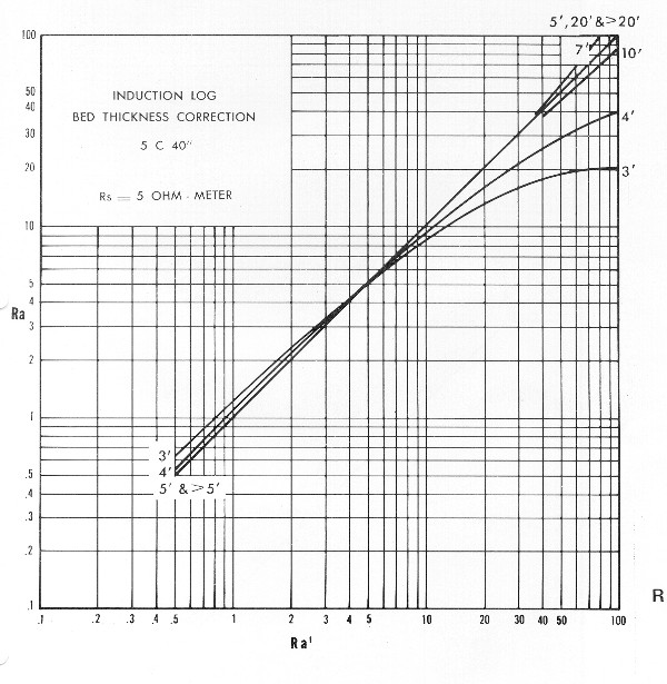
When the surrounding formation resistivity is 5 ohm-meters – less correction is necessary.

Given a 3 foot thick zone having resistivity of 4 ohm-meters and surrounding resistivity of 5 ohm-meters,

Using the Induction Log Bed Thickness correction chart for 5 ohm-meter surrounding formation;

Resistivity (Ra’) = 4 ohm-meters.

Bed boundary determination:

Bed boundaries occur at the inflection point of the induction resistivity curve. The inflection of the curve is the point at which a tangent line moving along the curve reverses direction.