PART
II, PAGE 1
DENSITY
TOOLS:
Density
tools are designed to measure bulk density of the formations in a well. The tool
is comprised of a “mandrel” made of very dense metal that allows collimation of
backscattered gamma rays and a “caliper” that is used to assert side-ways
pressure to force the density tool against the sidewall of the well. The
caliper also provides information about hole diameter. The density measuring
instrumentation in the tool usually consists of a gamma scintillation detector
and pulse conditioning circuits.
HOW DENSITY TOOLS WORK:
A
source of gamma radiation in the form of an encapsulated (sealed) gamma ray
emitting source is used. The source is commonly made of Cesium 137 or other
gamma ray emitter. Back-scattered gamma rays are collimated by a “window” in
the side of the tool. The gamma rays are sensed by a scintillation
detector. A scintillation detector uses
a scintillation crystal made of a material like thallium sodium Iodide. The
crystal converts incoming gamma rays into photons of light using a process
called “scintillation”. The photons of
light emitted by the scintillation crystal are detected by a photo-multiplier
tube. The photo-multiplier tube converts
photons into millions of electrons thru a “photo-electric process”. Gamma ray
photons remove electrons from a photo sensitive surface within the tube.
Electron multiplication occurs as electrons are produced and successive stages
of “dynode” electrodes within the photo-multiplier tube further amplify the
photon “pulses”. The resulting output is in the form of electrical pulses
representing the detected back-scattered gamma rays.
COMPTON
SCATTERING:
Gamma
rays emitted by a density tool source undergo several possible interactions
when they collide with matter.
In
the first interaction, at low energy, the photo-electric effect is the dominant
interaction. When low energy gamma rays collide with an atom and it’s energy is absorbed by the atom, a photo-electron is
emitted.
A
second interaction, at intermediate energy, the Compton effect is the dominant
interaction. The colliding gamma ray scatters (bounces) from an electron giving
up part of it’s energy. The energy of the scattered
gamma ray is a function of the angle of the collision. Each successive
collision results in reduction of energy until the gamma ray is absorbed by a
photo-electric interaction.
The
third possible interaction, at high energies, greater than 1.02 Mev., the gamma
ray is converted into an electron-positron pair. This interaction is called
pair production. The positron represents anti-matter. When it interacts with an
electron, they annihilate one another and produce two gamma rays. The two gamma
rays travel in opposite directions with equal energies of 0.51 Mev. These lower energy gamma-rays interact with
other atoms and are eventually subjected to
Gamma
ray sources containing Cesium 137 are low energy sources. The relatively low
energy of this source excludes the possibility of counting the results of pair
production making radiation intensity measurements only due to the effect of
BULK
DENSITY:
The
number of back-scattered gamma rays is directly related to the electron density
of the surrounding materials. Fortunately, electron density is very closely
proportional to bulk density for most low mass elements. The ratio of electrons per atom to atomic
weight is close to .500 . This ratio is referred to as the Z/A ratio.
re
= rb (2 Z/A)
Where: rb
= bulk density
re
= electron density
Z
= Sum of the electrons
A
= Total Atomic weight
Limestone: (CaCO3) Z/A = .500
Dolomite: (CaMg(CO3)2) Z/A = .499
Since
the intensity of the gamma source may be considered constant, the geometry of
the tool is also constant and the linear absorption coefficient for common
rocks is constant for the energy levels involved, the validity of using gamma
intensity as a method of measuring formation bulk density is established.
Counts
are inversely related to formation bulk density. High counts indicate low density, and lower
counts indicate higher density.
BOREHOLE
COMPENSATION:
Density
logging tools have a relatively shallow depth of investigation. The measurements are therefore subject to
effects of mudcake and borehole rugosity (diameter). To compensate for these
effects, a two detector density tool is used.
Two detectors having two spacings, short and long, with reference to the
source have count rates based on their respective distances from the
source. In an ideal borehole, the count
rates are known for a given tool design. A graph can be constructed having a
straight line (referred to as a spine) that represents the ratio of count rates
for various bulk densities. Additional lines referred to as ribs are plotted
representing deviations from the spine due to various mudcake densities and
thicknesses. Borehole compensation is
done thru computer calculation based on count rate deviation from the spine.
CALIBRATION:
Density tools are calibrated using
three blocks having known density.
Typical materials used for calibration
are, Aluminum (2.70 gm./cc), Magnesium (1.74 gm./cc), and Plexiglass plastic
(1.1 gm./cc).
POROSITY
FROM DENSITY:
Rearranging
the equation,
f
= (rma – rb) / (rma – rf)
Porosity
(f) can be calculated given bulk density (rb), if fluid density (rf) and matrix density (rma) are known.
Typical
matrix densities (rma)
are as follows:
Anhydrite 2.899 – 2.985 gm/cc
Dolomite 2.8 – 2.9 gm/cc
Kaolinite 2.6 – 2.63 gm/cc
Montmorillonite 2.2 – 2.7 gm/cc
Quartz 2.653 – 2.660 gm/cc
Typical
fluid density (rf)
of water is 1.0 gm/cc.
Formation
fluids containing oil and gas .7 gm/cc.
Formation
fluids containing gas .3 gm/cc.
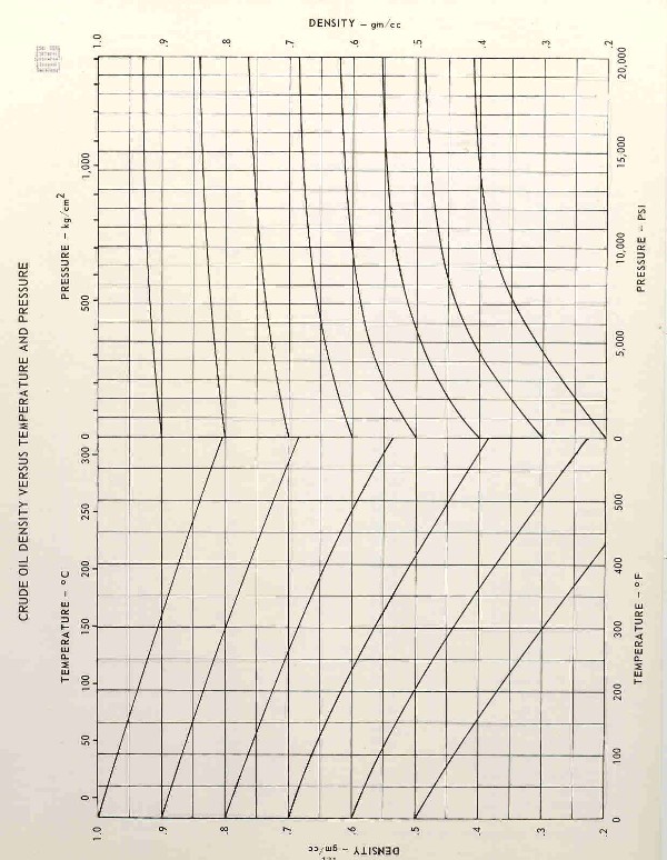
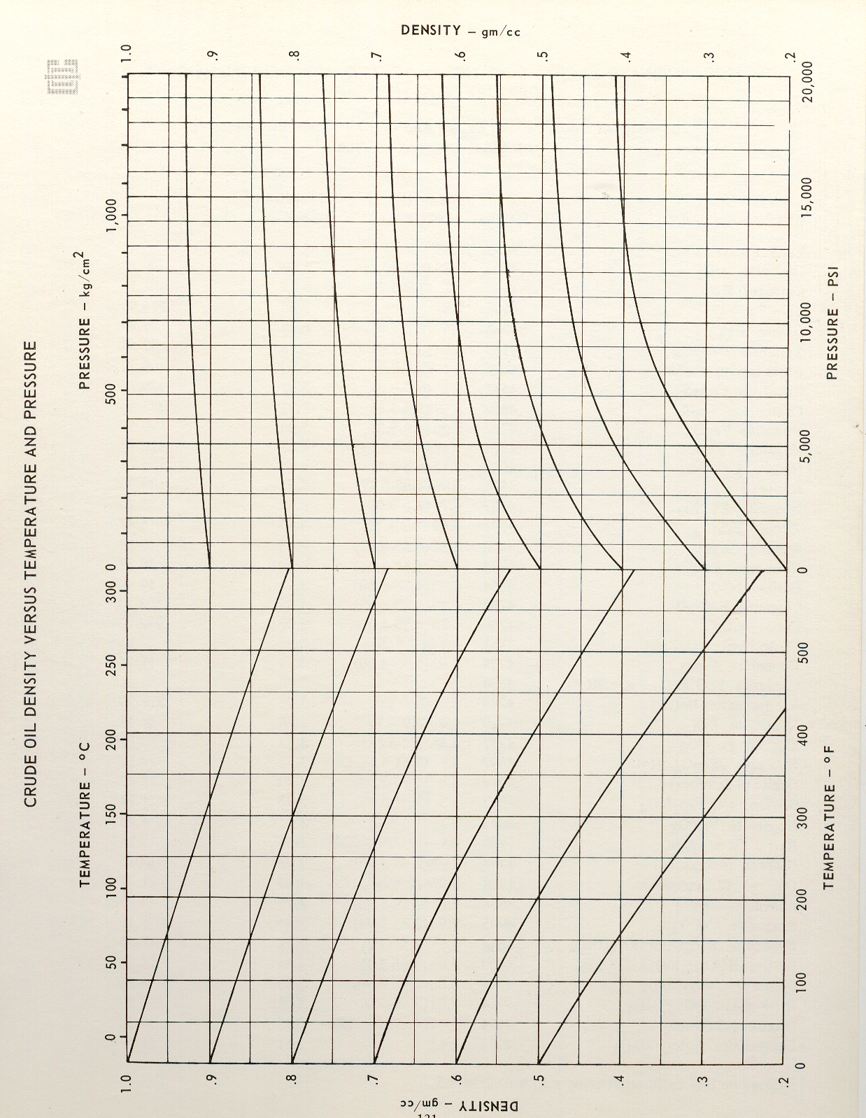
CORRECTION
FOR FLUID DENSITY:
Formation fluid may be freshwater, salt
water or other fluid. Because Density porosity is based on the assumption that
the fluid density is 1.0 grams/cc, it is important to correct for the effect of
temperature and pressure on fluid density.
Density versus temperature and pressure
for water and salt water:
Density correction chart for Crude oil
CORRECTION
FOR SHALE OR GAS:
The
physical properties of shale must be known in order to correct for the effect
of shale or clay in a sandstone matrix. Shale densities vary according to
depth. The range of shale density may
vary from 1.8 gm/cc near the surface to 2.60 gm/cc at 12,000 feet (US
Bulk
density in a laminated shaly sand is based on; shale density, matrix density,
and fluid density.
Laminated
shale-sands are defined as having laminae that do not exceed .5 inch thickness.
The calculation
is as follows: (not used in log interpretation)
rb =
rsh + rf
+ rma
rb =
(Vsh x rsh)
+ (f x rf) + (1 - f - (Vsh x rsh)) x rma
where Vsh = shale volume (percent
shale)
The calculation
for rma correction, rma(corr) is:
rma(corr) = (Vsh rsh) + (1-Vsh) rma
GAS
CORRECTION:
The
fluid density of a gas reservoir will be composed of a liquid fraction (SL) and
gas fraction (SG).
See a
chart of gas density.
The
corrected fluid density, rf(corr) is calculated as follows:
rf(corr) = SL x rL + SG x rG
See a
chart of the effect of gas and shale.
REVISED
11-24-2023 © 2003 - 2023 WELLOG All Rights Reserved