WELLOG LOG INTERPRETATION
SHORT DISCLAIMER:
Interpretation of data from well logs is
many times subjective. Depending on the accuracy of the log data and the
experience, proficiency, and care taken by the observer in the process of
interpreting that data, the possibility for error is very great.
Different approaches to log interpretation many times produce different
conclusions based on the use of more data or less data including more or less
“good” data. The following information is for informational purposes only. Any
application of the following information including equations is the sole
responsibility of the user. No representation is made to the accuracy and/or
completeness of this information. If errors are found, the reader is
encouraged to contact support@wellog.com
MEASUREMENT UNCERTAINTY:
When measurements of physical
properties are made, a certain amount of uncertainty prevails. Learn more about
uncertainty of measurements at http://www.physics.nist.gov/cuu/Uncertainty/index.html.
Learn more about uncertainty in well log analysis with
Monte Carlo simulation.
Here’s a link on the subject of units of measurement.
Links to Petrophysical consultants:
Ron Zittel www.rjzpetrophysics.com
WEBINAR:
WELLOG provides a free online Seminar on log
interpretation. It’s called a webinar. NEW Material
added every day!
INTRODUCTION:
The purpose of any Geophysical Log is
to provide meaningful information about the geological and physical conditions
in and around a borehole. Many books have been written on the subject of
log interpretation. Fundamental Log Interpretation has not changed in decades
and will probably not change.
Today, logging is most often performed
using digital data acquisition platforms. The data stored in a data file may
have extensive statistical computation applied to it. Intelligent systems apply
the same and sometimes better algorithms than their human counterparts once
did. The result is faster and often times “smarter” interpretation.
Taking the additional steps required to apply corrections to raw data and
perform ‘sanity’ checks on results adds confidence to any interpretation.
A WORD ABOUT CALIBRATION:
EVERY LOG should contain calibration information.
Interpretation can only be based on accurate and true measurements having a
verifiable reference. Ideally, calibration should be performed before and after
each log.
ELECTRIC LOG (E-LOG) INTERPRETATION:
Possibly the most important log that can
be obtained is an E-log. A properly
calibrated E-log will provide important information about formation Electrical
Resistivity. In addition to resistivity,
Spontaneous Potential (SP) is obtained. SP shows lithology and type of
lithology in terms of sand/carbonate or shale/clay and relative proportion of
each.
Electric Log operation is based on ohms law.
Ohms law
states: Resistance = V/I
Apparent Resistivity (ra)
takes into account the electrode geometry as follows:
ra = V/I x G
Where:
G = Geometric Factor (4pAM) AM is the distance measured (in meters) from A
to M electrodes.
V = Measured Voltage
I = Applied Current
View resistivity [Model].
View an E-log tool: [E-log tool]
Learn more about [electric log] applications.
Resistivity is usually measured in
units of ohms – meter2 / meter or; “ohm-meters”.
Electrical Resistivity provides
information about the fluid that is in the pore spaces within the rock matrix
in oil and water wells. Because electrical resistivity is controlled by
ion flow in liquids, the E-log will provide confirmation of the existence of
water, water quality, and/or hydrocarbon
content of the rock matrix. The electrode spacing (A to M) used on the E-log tool is directly related to the depth of
measurement. When multiple spacings are used, resistivities of different
depths are measured. It is possible to form conclusions on invasion and
permeability based on resistivity measurements made at two or more different
depths into the formation. See a tornado chart. If no invasion has
occurred, then both shallow and deep curves will read the same resistivity. If
invasion has occurred, then the shallow resistivity will reflect the resistivity
of the invading mud filtrate and the deep resistivity will reflect the
formation fluid resistivity. Resistivity curves should read the same and
depart only where invasion occurs.
In a water
well, higher resistivity in a saturated zone implies higher quality water. Total Dissolved Solids in water is related to the
resistivity of water. Although certain conditions apply, as Total Dissolved
Solids decrease, water resistivity increases. (Turcan, 1966)
In wells having hydrocarbons,
increasing resistivity in sandstone or carbonate zones may be an indication of
increasing hydrocarbon content.
The amount of fluid contained in a
formation is directly related to porosity.
Porosity affects formation resistivity. In water filled pore
spaces, as the volume of water increases, the capacity for more ions increases.
More ions mean more conductivity.
Conductivity and Resistivity are inversely related.
Conductivity is expressed in units of
micro-mhos per centimeter.
Conductivity ( C, in micro-mhos/cm) = 10,000/
Resistivity (in ohm-meters)
In the SI system of units, Siemens are
used to replace mhos. 1 Siemens = 1 Mho.
Learn more about [Siemens and Mhos].
Formation resistivity is affected by
three factors: Salt Concentration, Temperature, Pore volume (porosity).
Formation Resistivity Factor (F) is a
fundamental concept in log interpretation and analysis. The formation resistivity factor
is defined as the ratio of the electrical resistivity of a rock 100 percent
saturated with water to the resistivity of the water with which it is
saturated, (Archie, 1942).
The equation
is: F =
Ro/Rw
(Referred to as Archie’s Equation)
Given Rw = .05,
If Ro = 5.0 then F = 100
If Ro = 1.25 then F = 25
If Ro = .55 then F = 11
POROSITY FROM RESISTIVITY:
Archie found a relation of Formation Resistivity Factor
(F) to Porosity (f) as
follows:
F = a / fm
The constants (a) and (m) are related
to lithology.
Cementation factor (m) in a consolidated sandstone or a porous limestone is 1.8 to
2.0. In a clean unconsolidated sandstone values for (m) may be as low as 1.3
and the constant (a) is equal to 1.0.
An empirical formula based on studies
of core data from numerous localities has resulted in the equation:
Porosity of 10 percent results in a
Formation resistivity Factor of 100
Porosity of 20 percent results in a
Formation resistivity Factor of 25
Porosity of 30 percent results in a
Formation resistivity Factor of 11
Notice these three Formation
Resistivity factors are the same as previously calculated with F = Ro/Rw above.
Therefore:
Rearranging:
f = (1/Ro/Rw)1/2
Requirements for this method are 100 percent water saturation, Rw
is known and mineral conduction is not present.
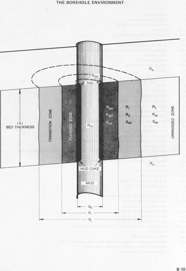
Using Shallow Resistivity from a pad
mounted measurement:
Given Resistivity of the flushed zone, Rxo and Resistivity of the
mud filtrate, Rmf, porosity may be obtained a follows:
f = (a Rmf/Rxo)1/m
where a = .62, m =
2.15 (From Winsauer et al., 1952)
PERMEABILITY FROM RESISTIVITY:
(From Alger 1966, Croft 1971, USGS)
A conclusion may be made that if deep and shallow measurements are
the same, that no invasion has taken place. If deep and shallow
measurements are different, then invasion has taken place. Invasion is an
indication that a rock matrix is permeable. It is because of the ability
of the E-log to measure fluid content, fluid quality, lithology, and indirectly
permeability, porosity and formation factor that make an E-log potentially the
most useful logging tool.
See the page on permeability.
CONSIDERATIONS:
All logging methods have limitations to
consider.
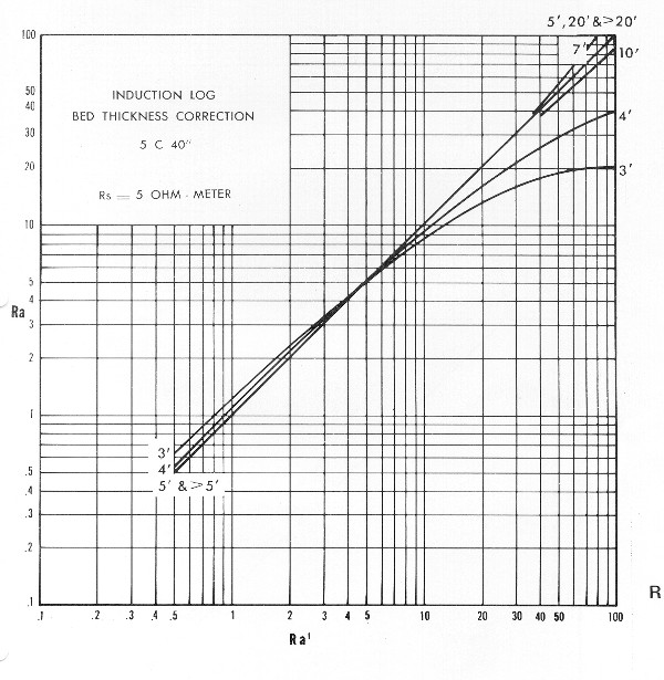
Bed thickness effect: The curves
produced by the normal devices are affected by bed thickness and
resistivity (Lynch 1962).
Where the resistive bed is more than
Although the radius of investigation
increases as the electrode spacing increases, the use of AM spacing greater
than 64 inches is not practical because thinner beds are not only shown at less
than true resistivity but may be recorded as conductive beds if their thickness
is less than or equal to the AM spacing.
Focused resistivity tools overcome this
limitation.
INVERSION METHODS:
Recently, software has been developed for improving resistivity
log interpretation. Old logs and new are being subjected to inversion
processing that removes the effect of surrounding formations. These techniques
will make electrical resistivity a more accurate viable logging method well
into the future.
OTHER RESISTIVITY METHODS:
The discussion thus far has been
related to resistivity using a “normal” electrode array.
Several other tools are available for
the purpose of measuring resistivity. Each tool is designed to provide an
accurate determination of formation resistivity in various borehole
environments.
Lateral resistivity measurements are used when it is
necessary to obtain deep formation resistivity measurements. Deep formation
resistivity is a close approximation of true resistivity where invasion is
small. In cases of deep invasion, interpretation must include a correction for
the invading borehole fluid. Note: Due to the larger spacing of electrodes used
in this method, thin formations are less noticeable on the log.
Focused electrode resistivity tools are used in
boreholes that have low resistivity mud or other drilling fluids. Normal and
lateral logging tools tend to conduct current thru the borehole fluid in this
case. Focused electrode systems are designed to reduce or eliminate
borehole fluid conduction. The current emanating from the tool therefore flows
into the surrounding formation and provides a more accurate measurement of
formation resistivity.
Micro electrode [wall] resistivity tools have small electrodes attached
to a non conductive pad that is pressed against the borehole wall while logging. These tools
are designed to measure the resistivity of the combined mud filtrate (Rmf) and
resistivity of the flushed zone (Rxo). The objective is to obtain information
about formation porosity and permeability. The small spacing used in the
electrodes make this tool very accurate in establishing bed boundaries.
Induction resistivity tools use
electromagnetic induction as a method of measuring formation resistivity. It is
important to know that all other resistivity measurements require fluid in the
borehole. Induction logging tools provide resistivity measurements in oil/water
and air.
Corrections are applied to all of the
above resistivity methods.
ACOUSTIC LOG INTEPRETATION:
An Acoustic Log (sometimes referred to
as a sonic log) when properly calibrated, will provide important information
about the physical structure of a rock matrix. The ability of sound to
travel within and through rock or sand and gravel depends on the physical
structure of the matrix. The amplitude, speed and phase relationships of
a transmitted sound wave that returns to an acoustic receiver is a function of
all of the combined matrix densities, interconnections, cementation,
fracturing, and porosities within the matrix.
Because the total transit time from the
transmitter to the receiver includes the path thru the borehole fluid +
formation + borehole fluid, Borehole compensated
(two or four receiver) logging tools are used. Borehole compensation
is accomplished mathematically by subtracting the borehole transit time.
Acoustic waveforms provide
information related to transit time (density) and amplitude (interconnection)
of the material comprising the rock matrix. Surface Geophysics has for
many years used seismic reflection and refraction for determination of
subsurface structure. Transit time (Dt) through sandstone, limestone, water, and other
materials have been determined in the laboratory. Relationships between
porosity and transit time are known. It is possible to determine porosity
of a given matrix if the transit time is known. Beginning with
velocity;
The bulk velocity is the sum of the
fluid velocity and the matrix velocity.
The relationship between bulk velocity
(vb) and fluid velocity (Vf) combined with matrix
velocity (Vma) becomes:
Given an equation referred to as the
Wyllie “time average equation”:
1/vb = f/vf + 1-f/vma
Transit time (Dt) is the reciprocal of velocity.
The equation for porosity (f) obtained from transit time (Dt) is:
f = (Dtlog – Dtma) / (Dtf – Dtma)
Where Dtlog = Measured Dt, Dtf
= fluid Dt, Dtma = assumed matrix Dt.
Fluid Dt is usually considered 200 microseconds per ft.
(Note some sources use 188 microseconds per ft.)
COMMON MATRIX VELOCITIES: (microseconds
per ft.)
MATRIX: VELOCITY:
Sandstone, unconsolidated 58.8 or more
Sandstone, semi-consolidated 55.6
Sandstone, consolidated 52.6
Sandstone, shaly 57 to 70
Limestone 47.6
Dolomite 43.5
Shale 62.5
to 167
Calcite 45.5
Granite 50.0
Gypsum 52.6
Quartz 55.6
Salt 66.7
Areas having fractures including
unconsolidated matrix can be inferred from an Acoustic Log.
CEMENT BOND LOG INTERPRETATION:
Acoustic logging is also used for
determination of cement bond in cased wells. This type of log is most often
referred to as a Cement Bond Log (CBL).
Acoustic signals propagated in steel
casing are observed to have large amplitude in free casing because much of the
energy is retained in the casing. Whereas the opposite effect is found in
casing that is in contact with a solid such as cement. The casing signal is
much smaller because the energy is coupled into the surrounding cement and
formation.
The thin plate velocity of sound in
steel is approximately 5300 meters per second (188 microseconds per meter).
A receiver having 3 feet spacing will
receive the casing signal (first arrival)
at 177 microseconds plus a short additional period allowing for transit time
thru the borehole fluid.
A receiver signal “time gate” is set at
the time of the expected casing signal. The casing signal will be the first
arrival at the receiver in free casing. The signal amplitude is recorded. A high signal amplitude indicates poor cement bond. A relatively low signal amplitude indicates good cement
bond. Amplitude is normally presented on a scale of 0 to 100 percent amplitude.
An area having no cement bond is represented by 100 percent amplitude. Due to
the fact that well cemented pipe can never reduce the signal to “zero”, a good
reference for zero signal is the best cemented portion of the cased hole. Using
information obtained from a Variable Density (waveform) display referred to as
a VDL display, it is possible to observe
the entire receiver wave train. When cementation is complete (
good bond) from casing to cement to formation, it is possible to observe
waveform shift in delta- time in the later arrivals that can be correlated to
open-hole acoustic delta-time logs.
CBL ATTENUATION:
The measurement of attenuation measured
in decibels (dB) is obtained from the amplitude as follows:
Attenuation = 20/D x Log10(A/Ao)
Where:
Attenuation is measured in decibels.
Ao is the transmitter amplitude measured in
millivolts.
A is the receiver amplitude measured in
millivolts.
D is the distance from the transmitter
to receiver (spacing) meters or feet as specified.
Note: Attenuation refers to the
reduction of amplitude. Therefore, attenuation is measured in terms of -
dB.
OTHER CBL TOOLS:
Sector bond tools (SBT), Radial bond tools
(RBT), and Ultrasonic Imager Tools (USIT) are other options available for
Cement bond applications including casing inspection.
GAMMA LOG INTERPRETATION:
Natural gamma radiation occurs in rock formations in varying
amounts. Uranium, Thorium, Potassium, and other radioactive minerals are
associated with different depositional environments. Sedimentary sandstone and
Carbonate environments are low in gamma radiation. Clay and Shale formations
exhibit greater amounts of gamma radiation. A log of gamma radiation in
“counts” or API units will give a positive indication of the type of lithology.
Interpretation of gamma log data is done based on the relative low and high
count rates associated with respective “clean” and “dirty” environments.
Composition of formations having more clay or shale as indicated by higher
gamma count rates generally are more tightly compacted with fine particles and
therefore have less porosity and permeability. Formations having high gamma
count rates even though they may exhibit low water saturation are generally
unfavorable for production in oil and water well environments.
It is important to be aware that
certain areas are known to have sandstone formations with higher than normal
levels of radiation. These formations are sometimes erroneously interpreted.
Information from an SP log can be used
for correlation.
Coal formations normally have very low (almost zero) gamma
radiation and contrast quite well with surrounding formations. Knowledge of
local “exceptions” is an important aspect of accurate interpretation.
GAMMA LOG CALIBRATION:
Gamma radiation is detected differently in every logging tool. Due
to variation in detector types, tool design, detector efficiency and overall
tool response, the American Petroleum Institute (API) standard of API Units is
commonly used for calibration. A Test well located in Houston, Texas has been
used for many years as the API reference test well. The well is designed with
three layers of concrete. The top 8 feet of concrete is low radiation, the
middle 8 feet is a mix of radioactive elements designed to closely match a
radiation level of twice the mid-continent US shale, and the bottom 8 feet is a
low activity concrete zone. A tool is calibrated in the test well by first
measuring the gamma radiation counts in the low radioactivity zone which is
considered to be 0 API units. A second measurement of gamma counts is the made
with the detector centered in the high radioactivity zone. The high
radioactivity zone corresponds to 200 API units. Secondary reference
calibration jigs containing a low-level gamma radiation source are often used
in the field to establish detector calibration. Operation of the detector is
confirmed by placing the source at a specified distance from the detector, and
then at a distance sufficiently far away to obtain background
counts.
NEUTRON LOG INTERPRETATION:
A Neutron Log when properly calibrated
(usually to an API standard) will provide important information about the
content of the pore spaces within a rock matrix. Neutrons emitted from a
neutron source are slowed down and eventually captured through interaction with
hydrogen atoms. Once captured, a gamma ray of capture is created.
Neutron Logging tools are designed to respond to slow Thermal
Neutrons or Gamma Rays of Capture.
Since hydrocarbons and water (H20)
contain hydrogen a neutron log will provide knowledge of the hydrogen in the
pore spaces of the matrix. When more hydrogen is present, more neutrons
are captured, and fewer neutrons reach the neutron detector. Conversely,
lower porosity, neutrons travel farther and reach the detector, increasing
neutrons counted at the detector. In other words, increased fluid filled porosity is indicated by lower neutron count.
Neutron
porosity is calculated based on neutron tool response in known lithologies having known porosity.
Tool response is specified in terms of American Petroleum
Institute (API) units. The standard unit for neutron logging tools is the “API
Neutron Unit”. 1000 API units is assigned to any
neutron tool in a water filled hole having 7 - 7/8 inch diameter in Indiana
Limestone of 19 percent porosity. One API Neutron Unit is 1/1000 of the
difference between tool instrument zero and the log deflection in the Indiana
Limestone section. The API test well is
located at the University of Houston, Houston, Texas.
When a tool is calibrated at the API test
well, its response to a standard neutron calibrator is also determined. The
differential deflection produced by this two environment device is compared to
the API test well deflection representing 1000 API Units. A definite number of
API units can then be assigned to a tools calibrator deflection. This
calibration figure must be determined for each model or series of tool.
Each tool supplier develops a transform
from API units to porosity for the neutron tools they produce.
The general equation is: Porosity
(f) = natural log (API Log
counts * constant + constant)
Neutron Porosity is based on a
Limestone matrix (Indiana Limestone).
A correction to obtain porosity for a
sandstone matrix is: Porosity (fss) = 0.95 (f(n)) + .035
DENSITY LOG INTERPRETATION:
A Density Log when properly calibrated
will provide reliable information about matrix bulk density. When density
is known and a specific matrix is assumed then porosity of the matrix may be
determined. A mathematical relationship exists between measured density,
assumed matrix density with no porosity and the density of the material filling
the pore space. Water has a density of 1 gram per cubic centimeter.
Sandstone with no porosity has a density of 2.65 grams per cubic
centimeter. If a sandstone matrix is assumed for example, then a given
density of 2.00 grams per cubic centimeter allows calculation of 40 percent
porosity.
The equation for porosity (f) obtained from bulk density is: f = (rma – rb) / (rma – rf)
Where rb = Measured bulk density, rf = fluid density, rma = assumed matrix density.
For reference, Sandstone has a density
of 2.65 gm/cc, Limestone is 2.71 gm/cc, Dolomite 2.87 gm/cc.
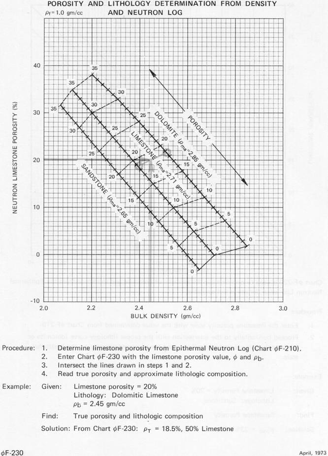
NEUTRON – BULK DENSITY CROSS-PLOT:
Combination of data from a Neutron Porosity Log and Bulk Density
log can be helpful in identification of Lithology. A chart is used that has the
known relationship between Neutron Porosity and Bulk Density for three
matrices; Sandstone, Limestone, and Dolomite. It is possible to determine ratio
of Sandstone/Limestone and obtain a more accurate porosity using the cross-plot
chart. Results from the cross-plot chart should be correlated with known
lithological information.
Neutron porosity and density porosity are often presented in an
overlay on the same scale on a log for shale and gas identification.
View a neutron-density cross-plot chart.
Cross plot methods are treated extensively in the WELLOG webinar.
AN ADDITIONAL BENEFIT:
If the Lithology is known to be a Sandstone
and the cross-plot shows a Dolomite, then it is possible one or both sets of
log data are not properly calibrated. If the cross-plot shows correlation, then it provides a closed loop between logging
tool response and lithology.
SHALE VOLUME CORRECTION:
Porosity data should be corrected for shale content in the zone of
interest. Porosity values are
optimistic when shale is present.
Depending on the value of Rmf/Rw, either the natural
gamma data or SP data is used to determine shale volume.
Correction
for shale is covered extensively in the advanced pages of the WELLOG
webinar.
FORMATION EVALUATION:
After the appropriate corrections are applied, a realistic
Formation Evaluation can be made. It should not be under-estimated that many
corrections are required to properly analyze a well log.
WATER SATURATION:
One objective in Log Interpretation is
the evaluation of a petroleum formation for water saturation (Sw). If it
assumed that only two types of fluid occur in the formation, for example oil
and water.
The calculation for water saturation is as
follows: Sw = (F * Rw / Rt)1/n
Where n is the saturation exponent (usually a value of 2).
The oil saturation as a percent of the pore space
is simply: So = (1 – Sw)
WELLOG has an extensive log interpretation library and personnel with experience in log
interpretation.
WELLOG will
provide answers to your log interpretation questions free of charge!
WELLOG will
provide training on Logging and Log Interpretation.
WELLOG is currently sponsoring a Web based Seminar called a “Webinar” on
Log Interpretation Fundamentals.
As with most of the WELLOG website,
improvements and additions occur every day.
Registration in the webinar is
voluntary. Email training@wellog.com with Name, Company,
and your interest in log interpretation.
If you need more information or links
to other resources contact support@wellog.com